Technical research note
How simulation size changes a housing stress test
Bottom line
Across 64 simulations, the early sale index response changed with population size and became less noisy. Even the largest baseline still drifted. This is a numerical study of a model with inherited assumptions, while national calibration continues.
The experiment
The size of the simulated market matters
A housing simulation represents households making decisions, borrowing, moving and trading with one another. Changing the number of simulated households can change both the amount of random variation and the way the market behaves. A result from a small population should therefore be checked at larger sizes before it is used to support a wider claim.
We completed 64 full simulations at populations of 30,000, 100,000, 300,000 and one million synthetic households. Each size used eight independent seeds. Every seed produced a baseline and a matching scenario, giving eight pairs per size and 32 pairs overall.
Each run lasted 600 model months. At month 360, the scenario received a one percentage point upward impulse to the new lending rate. The bank then continued its endogenous rate updates. Existing mortgage contracts were retained. This was a change to new borrowing costs, rather than an exercise in which every outstanding mortgage repriced together.
The 50 years are synthetic model time. They are not a reconstruction of 50 observed years or a forecast beginning today.
Paired results
The early estimate changed as the population grew
Over the first 12 months after the impulse, the mean sale index response was +0.1618 percentage points at 30,000 households, with a Monte Carlo standard error of 0.2141. At one million households the mean was −0.65465 percentage points, with a standard error of 0.10438.
The small positive estimate is smaller than its own standard error. It does not establish that the impulse raised prices in a small model. The larger population produced a more precise negative estimate under this model and these assumptions. It does not establish what would happen to real house prices.
The result is a difference between changes, each measured from its own paired pre event mean. It is not a change in the Bank Rate or a direct forecast of the percentage fall in national house prices.
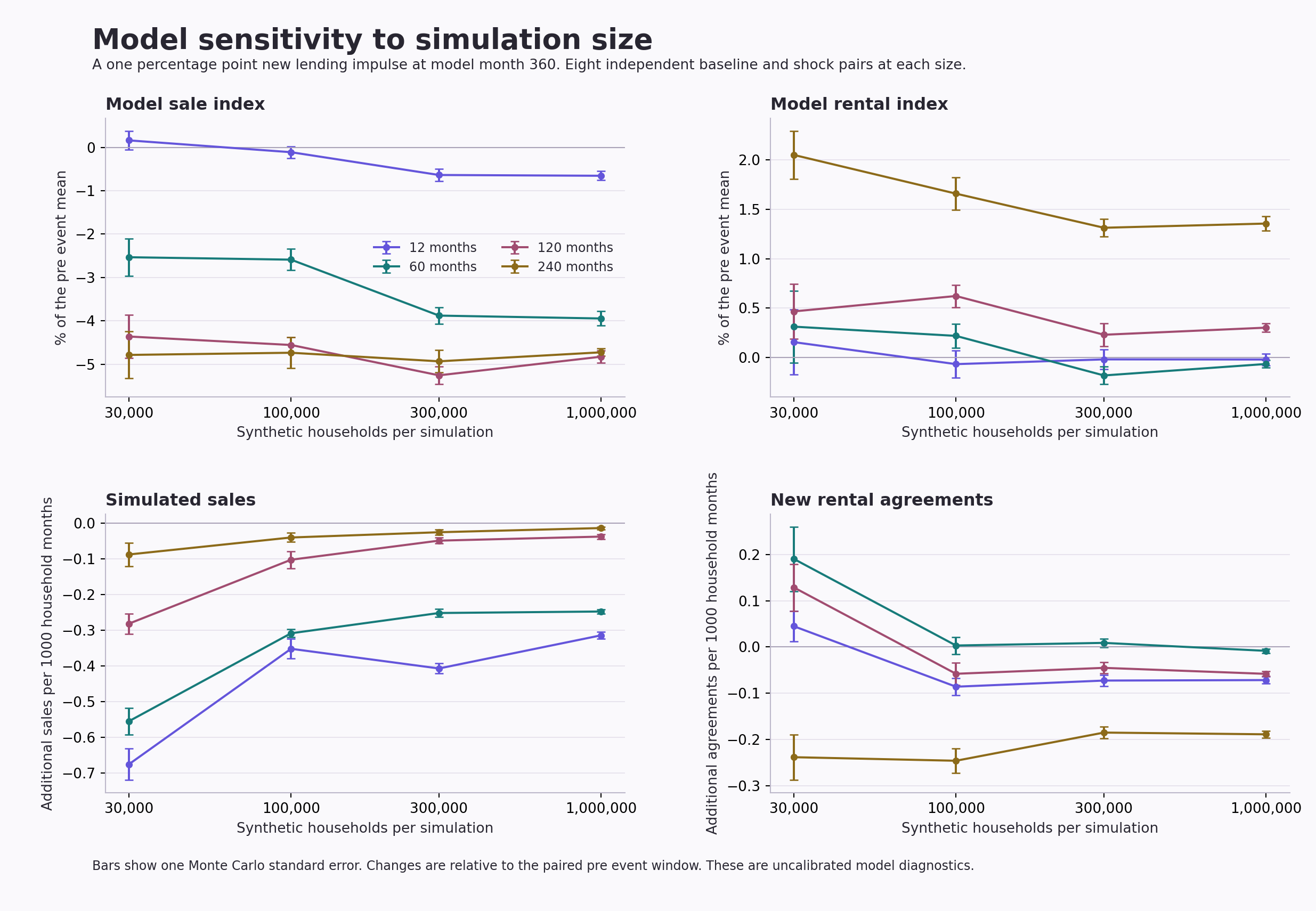
The difference also appeared beyond the first year. Over the first 60 months, the sale index mean was −2.5336 percentage points at 30,000 households and −3.9466 at one million. Longer windows average the whole period from the event, so the 60 month figure is not the value at month 60.
The larger sizes do not move monotonically towards one answer at every horizon. Similar estimates at two sizes would not by themselves prove convergence. The charts also show rental indices and market activity because a price index alone cannot describe the adjustment of the simulated market.
The baseline check
A larger market did not become a settled market
The unshocked baselines continued to move. At one million households, the mean sale index rose 18.2994% between the 60 month windows ending at model months 120 and 240. It then fell 8.0673% between the windows ending at 240 and 360. The corresponding Monte Carlo standard errors were 0.3223 and 0.3436 percentage points.
Later baseline comparisons were smaller but remained nonzero: −1.0937% between the windows ending at 360 and 480, then +1.0105% between 480 and 600. Those changes had standard errors of 0.2953 and 0.2633 percentage points.
Each window contains the preceding 60 model months. These comparisons are changes between window means, not differences between single monthly observations. A fixed period allowed for the model to settle does not demonstrate that its economic dynamics have settled.
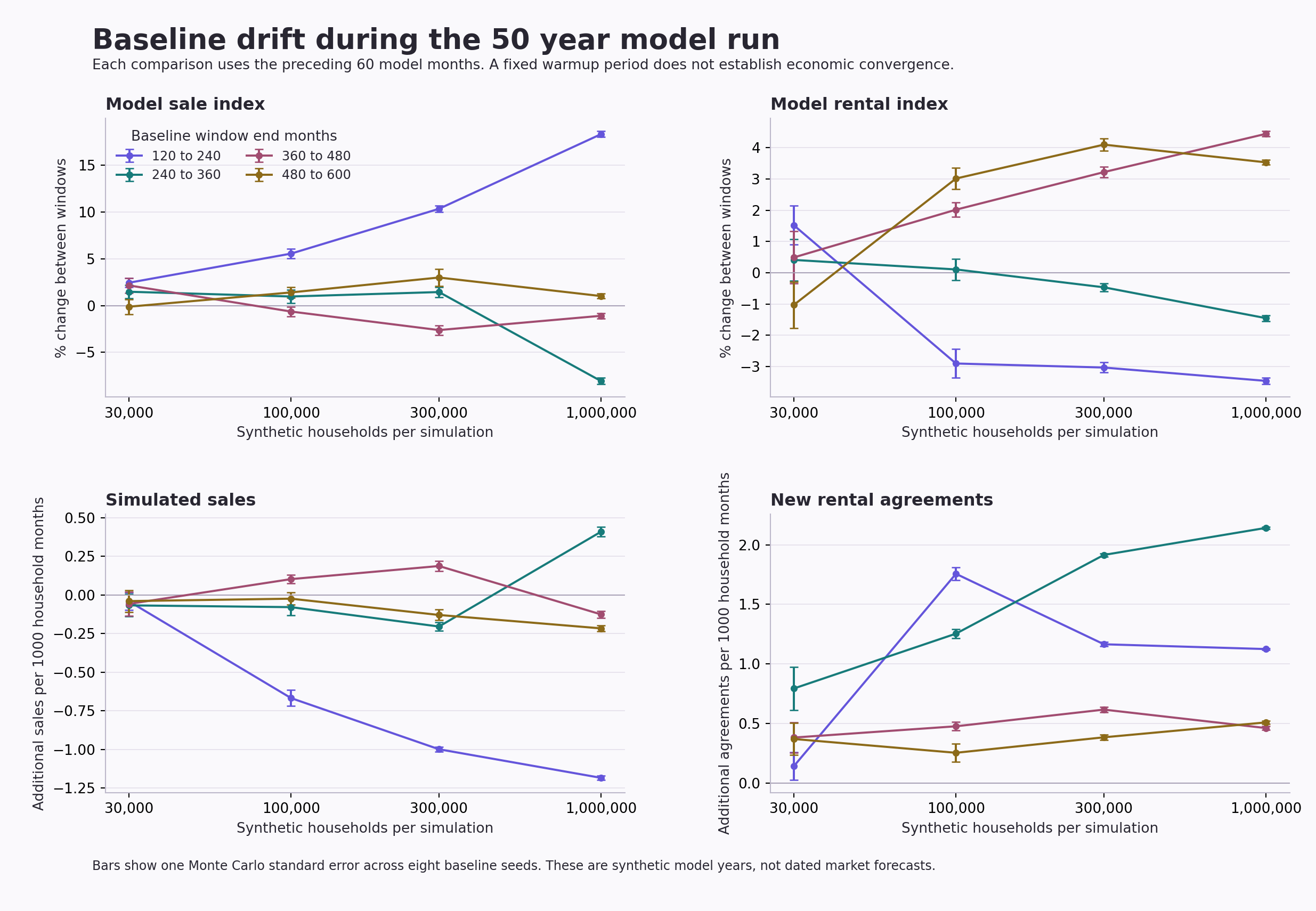
This matters for interpreting the scenario. Comparing each run with its paired baseline helps distinguish the impulse from the model’s own trajectory. It does not make that underlying trajectory an empirically validated description of the housing market.
Method and uncertainty
What the comparison measures
Within each pair, the initial seed, configuration and recorded initial state matched. Every saved regional and national output before the event was checked for exact agreement. Different pairs and population sizes used independent seed streams. After the impulse, economic decisions can change how random draws are consumed, so matching later random innovations is not claimed.
The reference period is model months 300 through 359. The first response window is months 360 through 371. The longer windows run from month 360 through 419, 479 and 599 respectively.
For an index, the paired response is 100 × [(scenario post event mean ÷ scenario pre event mean) − (baseline post event mean ÷ baseline pre event mean)]. We calculate this separately for each seed pair, then report the mean, the standard deviation across pairs and the Monte Carlo standard error. The latter is the standard deviation divided by the square root of eight.
Model sale and rental index summaries use geometric means, with fixed Census household weights across the 331 retained areas in England and Wales. Every required area and month must have a positive index for that measure to be reported. Transaction weighted mean sale prices and new agreement rents are separate measures in the download and remain sensitive to the mix of homes trading.
The error bars describe variation across these eight independently seeded experiments at each size. They do not include uncertainty about parameters, household behaviour, the empirical calibration or the future market. The four horizons and four sizes are diagnostic comparisons, not a search for a statistically significant result.
Model and scope
What this release cannot prove
The experiment uses our retained regional adaptation of the INET housing model at a pinned source revision. The original research is described by Baptista and colleagues in Bank of England Working Paper 619, Macroprudential policy in an agent based model of the UK housing market, published in 2016.
All 64 runs used the same model source, revision 520d75733ef3eca70a3526b1cad0d1b102c84d8d, and inherited older age, income, wealth and initial price distributions. Contemporary local tenure margins remained comparison targets. Later empirical controls and financial inputs being prepared for the national study were not part of this experiment.
The 331 area labels and weights do not establish that local income and wealth, tenure, housing stock, household movements or mortgage exposure have been calibrated to those places. Historical fit, geographic holdouts and the calibration of behavioural assumptions remain separate work. This note is finished evidence about numerical sensitivity, not the finished national housing stress test.
The simulations ran as Java workloads on the ARM CPUs of Isambard AI. The median elapsed time per million household run was 858.6 seconds, about 14.3 minutes, and the largest recorded process peak memory at that size was 5.99 GiB. These are measurements of these runs, not a general performance guarantee. The experiment did not run a full housing model on a GPU.
The practical lesson is to report population sensitivity and baseline drift alongside a stress result. More simulated households can reduce random variation while leaving important model assumptions and economic dynamics unresolved.
Open research files
Inspect the results
The national paired effects CSV contains 128 aggregate rows across four population sizes, four response windows and eight measures. It retains the planned and observed pair counts, missing pair counts, means, standard deviations, Monte Carlo standard errors and units. The baseline drift CSV contains 128 rows with the same eight measures and the two window endpoints for each comparison.
The resource summary CSV records the 16 runs at each size, their minimum, median and maximum elapsed times, and the largest observed process peak memory. It does not state a compute charge or an award balance. The file manifest records the exact source revision, definitions and SHA256 hashes. The national label means an aggregate of the synthetic regional model, not a national statistical estimate.
The two charts may be downloaded at their original resolution as the population response chart and the baseline drift chart. Please cite this note when using its results.
Suggested citation
Upgraded Intelligence (2026), How simulation size changes a housing stress test, version 1.0, UI-MOD-SIZE-2026-01.
For research enquiries, corrections or an accessible extract, contact hello@theupgradeauthority.co.uk. For observed local evidence, explore the UK Property Atlas or browse the research library.