Housing research on Isambard AI
Housing stress atlas for England and Wales
Bottom line
In 63 areas, simple benchmarks beat the simulation. Carrying forward the previous rent trend missed by 2.7 percentage points on average, compared with 7.7 for the model. Assuming sale prices stayed flat missed by 3.0 points, compared with 10.6 for the model.
- Scenario simulations
- 336
- Areas on the map
- 331
- Areas tested with real data
- 63
- Months of observed outcomes
- 24
Scenario explorer
Explore the simulations
The selected results could not be loaded.
Model response map
Housing model responses
Loading results.
Choose an area
Not availableMean model responseRange across runs ● Mean response
No result is loaded for this selection.
Each area is measured against its own unchanged control. The range describes variation across simulation runs.
Time after intervention
Compare response windows
The windows overlap. Choose one to update the map.
Boundaries from May 2022. Census reference date 21 March 2021.
Jan 2024 to Dec 2025
Model vs real market
We compared the simulation with two years of recorded rents and sale prices in areas whose local rent and sale outcomes were kept out of the new runs.
Change since Dec 2023
Basildon
How to read the comparison
Each line starts at its own December 2023 level. The previous trend carries forward the change seen over the preceding year. Percentage point errors compare changes, while the error in levels uses the original pound values.
The shaded band shows the middle 80% of repeated runs with the same rules and different randomly generated starting households. It measures how much the results varied between runs.
The new test uses the area split from the original study. That study already checked how its model fitted rents in these areas. The new runs leave out the local sale prices and rents scored here.
The official price series adjust for the mix of homes. The simulated averages reflect the sales and rental contracts the model generated. The model run with observed mortgage rate changes uses rates recorded after the starting date.
What the test tells us
The model tracked rent changes more closely than both benchmarks in three of the 63 areas. For sale prices, one or both benchmarks came closer in every area. Even when we supplied the mortgage quote changes that actually happened, the model's average errors in rent and sale price changes grew slightly.
The published atlas settings came closer to actual prices in pounds than the original settings did. Those settings were fitted using later data and still missed the change in sale prices by 9.8 percentage points on average. We repeated the price check using recorded transactions directly and the flat benchmark still came closest. Download the recorded sales comparison.
Use the atlas to see how the model responds to a change in rates or incomes. Evidence from this test favours the simple benchmarks for estimating how much local rents or prices will move.
We completed 336 housing market simulations on Isambard AI. The main panel contains 272 worlds, with one million simulated households in each. Seventeen scenarios were repeated with sixteen independent starting seeds. A further 64 worlds test four core scenarios at populations of 300,000 and three million households, with eight runs per case.
The interactive atlas covers the original 331 England and Wales model areas in the main panel, with results for sale prices, rents, turnover, tenure and empty private stock. The separate population comparison below shows where the answers change as the model gets bigger.
Higher quotes, fewer model sales
Increasing the annual rate quoted on new loans by one percentage point reduced the first year mean sale price by 2.31% against the unchanged control. The annualised sale rate fell by 6.49%. Both responses were negative in every one of the sixteen runs.
The sale mean response ranged from a fall of 1.37% to a fall of 2.99%. That range measures variation across the repeated simulations with fixed model assumptions. It is not an interval for what actual house prices will do.
The rate change applies to newly offered lending. Existing mortgage contracts retain their agreed payments and rates. The model then continues to set lending quotes through its bank pricing rule, so the initial change and the later realised quote path need to be read separately.
An income cut changes rents and turnover
Reducing the nonrental income input multiplier by 10% lowered the first year mean rent on new agreements by 7.53%. The mean across active private rental contracts fell by 2.77%. Both rent responses were negative in all sixteen runs.
The sale market produced a different initial pattern. Its transaction weighted mean rose by 5.01%, while the sale rate rose by 27.35%. Both increased in every run. A rise in the average price of the homes that traded does not establish that an unchanged home became more valuable. Transaction means also depend on which homes sell.
The direction changed over the longer horizon. In the twentieth year of the sustained income reduction, the model sale mean was 8.26% below its control and the active contract rent mean was 11.84% lower. These results make the response window and the measure important parts of the finding.
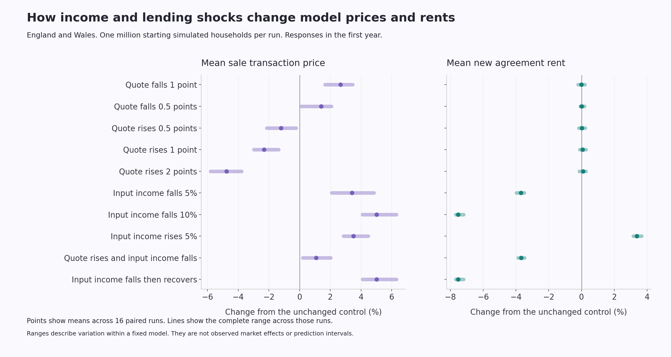
National scenario responses in the first year. Points show the mean paired response and bars cover all sixteen runs. View the full size chart or download its figures.
Follow the path as well as the starting shock
The lending experiment changes a quote at the start of the comparison. The income experiments change a multiplier applied to the model's nonrental input income. They are distinct interventions, with different effects on household decisions and market activity.
A separate recovery case restores the income multiplier after twenty four months. It gives a comparison with the sustained reduction while preserving the market history already generated. Applied income can also reflect changes in the model population and its income floors.
The chart shows the mean quote and income paths used in these comparisons. Its horizontal axes measure elapsed model time. They do not represent forecasts for named future calendar years.
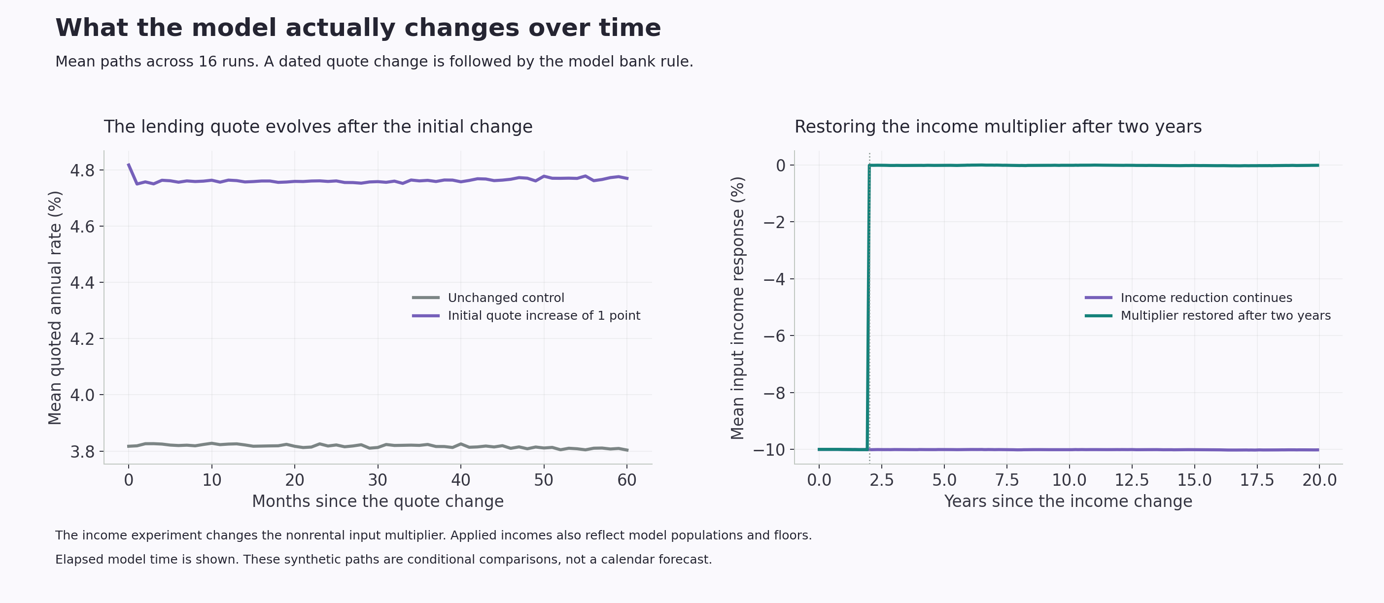
Mean input paths across sixteen runs. The recovery case restores its multiplier after two years. View the full size chart or download its figures.
What changes when the model gets bigger?
The first year sale mean response to a one percentage point increase in new mortgage quotes was a fall of 2.11% with 300,000 households, 2.40% with one million and 2.49% with three million. The direction persisted, while the range across runs became narrower.
Other results changed more. Under the 10% income input cut, the first year sale mean rose by 2.25%, 4.98% and 6.55% at those three population sizes. The new agreement rent mean fell by 6.69%, 7.52% and 7.80%. With a one percentage point quote increase and a 5% income input cut together, the sale mean moved from a fall of 0.40% in the smallest model to a rise of 1.92% in the largest.
This comparison uses eight runs per case at each population size, with seed labels 4001 through 4008. The main atlas and the other charts use all sixteen runs at one million households. That is why, for example, the income cut's one million household sale response is 4.98% here and 5.01% in the main panel.
Matching seed labels across different populations does not establish matching random outcomes. These results show sensitivity to population size. They do not establish convergence, and increasing the number of simulated households does not by itself correct the baseline's price or rent errors.
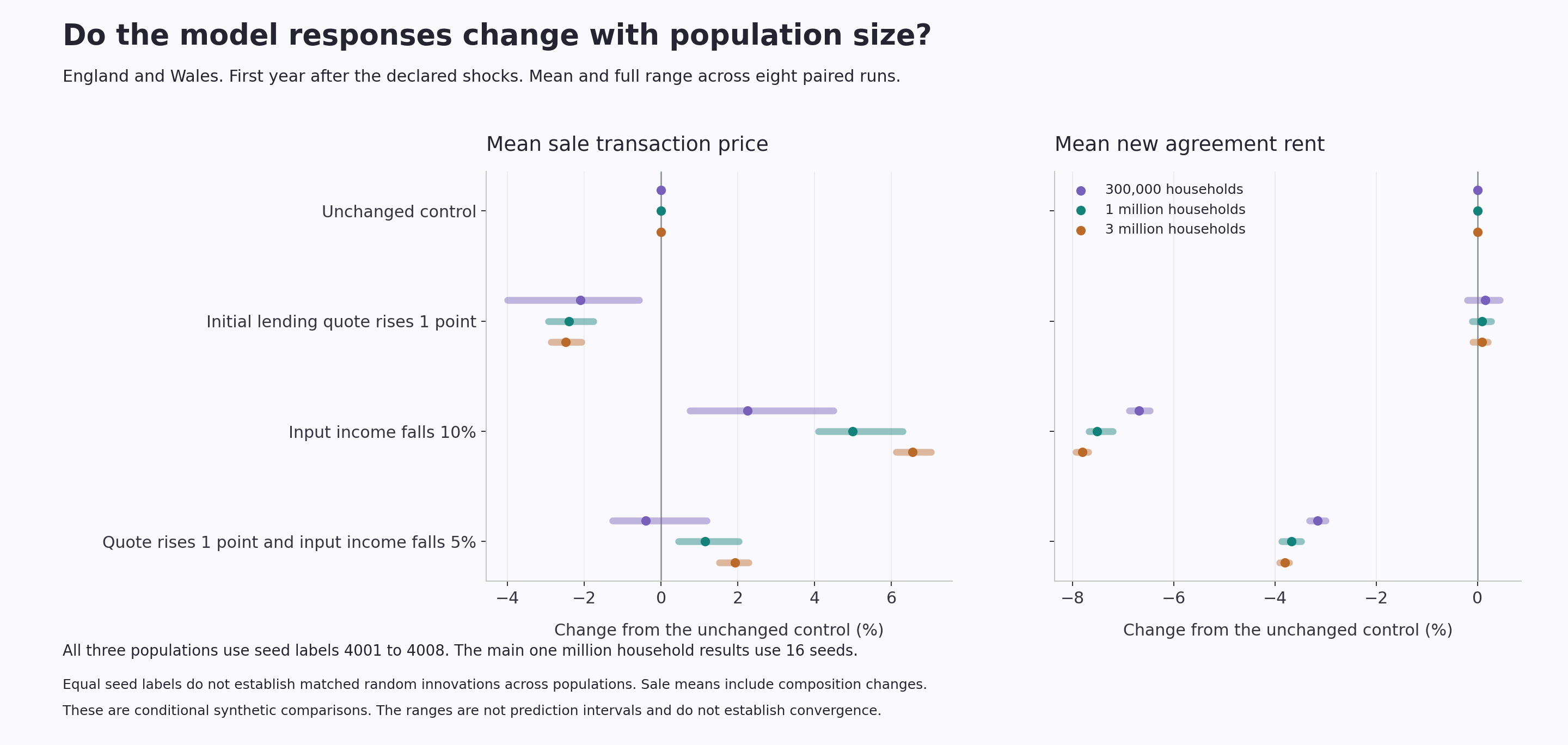
Population comparisons across four core scenarios. View the full size chart or download its figures.
Read each area against its own control
The atlas retains every original model area. National income cases change the input across all 331 areas; local cases change one selected area's multiplier. Each map result compares that area's scenario with its unchanged control, then summarises the valid paired runs.
A percentage change in a sale or rent mean differs from a percentage point change in a tenure share. The atlas states the unit for each measure. Where a denominator does not support a defined comparison, the result remains unavailable rather than becoming a zero change.
The national sale mean pools transaction values and counts inside each simulated world. It is not a simple average of the local price means. The same distinction matters when comparing national results with individual areas.
How the experiment was built
We built a geographical extension of the open housing model developed by the Institute for New Economic Thinking at Oxford with the Bank of England. Its original design is described in Bank of England Working Paper 619. The extension, conditioning and simulations reported here are Upgraded Intelligence's work.
The model contains interacting buyers, owners, renters, investors and a shared mortgage market. Household and tenure context comes from Census 2021. Supplied area income means refer to April 2022 through March 2023, and the retained national sale calibration target uses standard recorded residential transfers from 2025.
Parameters and controls were frozen before the final scenarios. Each world ran for 600 monthly observations, with 360 months before the intervention and 240 afterwards. Matched starting seeds and unchanged pre intervention records qualify the paired comparisons. After the intervention changes decisions, later random outcomes can diverge between a scenario and its control.
We report the mean of the individual paired responses. For a price or rent mean, each valid run's response is its scenario level divided by its control level, minus one. Tenure shares use percentage point differences. The downloadable figures retain the levels and denominators alongside the responses.
Download and cite the research
The main figures download contains 158,032 area and national response summaries, exposure summaries and monthly national traces. The detailed paired levels download retains all 2,528,512 declared area, window, measure and seed contexts, including explicit unavailable states.
The data manifest records file hashes, model identities and source context. Map boundaries are from May 2022 and retain the original model codes. The Census reference date is 21 March 2021.
Please cite Upgraded Intelligence when using these model results. Research and media enquiries can be sent to press@upgradedpm.com.
What this release cannot prove
This study covers 336 completed model worlds. The map presents 272 worlds with one million simulated households each. Separate population comparisons cover 300,000, one million and three million households.
The figures describe conditional model responses and do not establish forecasts or causal effects in the observed housing market.
Time in the atlas is measured in elapsed model months.
The baseline has substantial calibration errors. In the prior reserved calibration assessment, the simulated sale mean was £280,498 against a retained 2025 transaction target of £372,946, a gap of 24.8%. Median absolute rent level errors were 34.2% across 249 fitting target groups and 38.3% across 63 excluded groups. Those excluded geographical evaluations had previously been examined and are not fresh validation.
Inputs have different reference dates. Supplied area income means are conditioning data, so agreement with them is not an independent income prediction. The model does not identify a contemporary joint distribution of household income, wealth, debt and mortgage reset exposure. The 2025 sale target covers standard residential records and has incomplete registration coverage.
Sale transaction means include changes in the mix of homes that trade. The initial income case therefore does not establish rising constant quality house prices. The geographical extension does not model household migration or cross area housing search. Responses outside the directly changed area are not validated estimates of real geographical spillovers.
The experiment changes new lending quotes rather than repricing every existing mortgage. Fixed rate reset exposure and a separately calibrated rental supply response remain outside this version. Its residual housing category is a model placeholder, not a measured homelessness or social tenancy outcome.
The run range and standard error describe variation under one fixed set of model assumptions. They do not capture every uncertain parameter or provide a prediction interval for the real market. Paired worlds share their starting conditions, while later random outcomes can diverge after a shock. Population checks changed some response magnitudes and one mean's direction. They do not establish convergence across model sizes.
Suggested citation
Upgraded Intelligence (2026), Housing stress atlas for England and Wales, version 1.1, UI-HSG-STRESS-2026-01.